Rock Analyst Software application Rock Analyst Software application
User Manual version: 1.0
Name of software: Rock Analyst
Latest release of the Rock Analyst Software: 2.0
Developers: Dávid Farics, Éva Farics
Contact address: Éva Farics, Eötvös Loránd University, Department of Physical and Applied Geology, H-1117 Budapest, Pázmány P. stny. 1/C., Hungary. Email: eva.gyorfy@gmail.com
Year first available: 2016
Programming language: C#
Program size: circa 160 KB
Hardware and software required: PC with Windows operating system (XP or newer)
Screen resolution: min. 1024*768.
You can download the latest release of the Rock Analyst Software from this webpage and unpack the files locally.
The folder contains the following files:
Do not delete the files from the folder!
If you want to remove the application, you delete the folder.
Before the using you have to scan a cut surface of the rock or a thin section. The resolution of the scanning is minimum 300 dpi! The application uses only the characters of the English alphabet! We have to name the picture and later the file accordingly.
New image:
File > Add a new image (Ctrl + N)
It is important to select the picture from your computer (and not from a storage media).
Save the file:
File > Save as (Ctrl + Alt + S)
You have to save the file (*.txt) in that folder, which have also the picture. Without this step you cannot open the file the next time. Later you can move the folder on your computer.
Open the txt file(s) (one or more):
File > Open file (Ctrl + O)
If you open more than one file, you cannot create or modify curves. In this case you can use only the menu of calculations.
Close the file:
File > Close file (Ctrl + W)
Close the program:
File > Exit (Alt + F4)
At first you have to define the examined rock types (rock.dat file in the folder).
Tools > Rock Types (Ctrl + T)
You can name the rock types and can give a colour for them (Figure 1). Do not forget save the changes. You can modify the names and the colours whenever. The change of the name is available with double-click on the name.
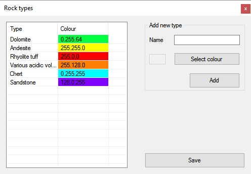
If you start a new project, and the rock types are different than before, you have to do another table. Important to make a copy from the former rock.dat file.
New curve:
Tools > Add curve (Ctrl + G)
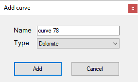
You can write the name and select the rock types of the curve (Figure 2a). Then you can draw round the clasts on the picture. You can edit the shape of the outlines (Ctrl + "click" on the outline). Furthermore, you can use the following with the curve:

You can use the ruler (2 mm) to determine the approximate size of the clasts:
Tools > Ruler
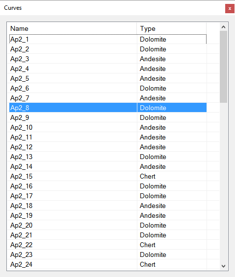
After the drawing you can see all of the curves in the menu item of Curves (Figure 3). Double click on a row of the list to select a curve. If something is wrong (for example the curve has only two point), the row is red.
You can see the results as follows in the menu item of Calculations (Figure 4):
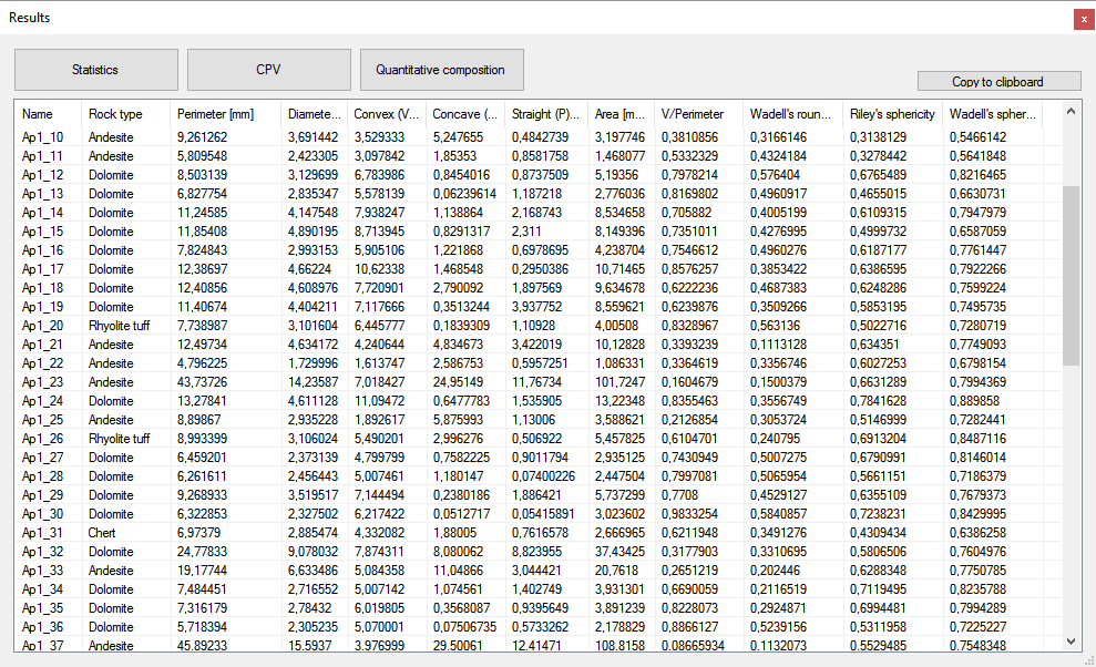
You can copy the table to clipboard (and paste into an excel document).
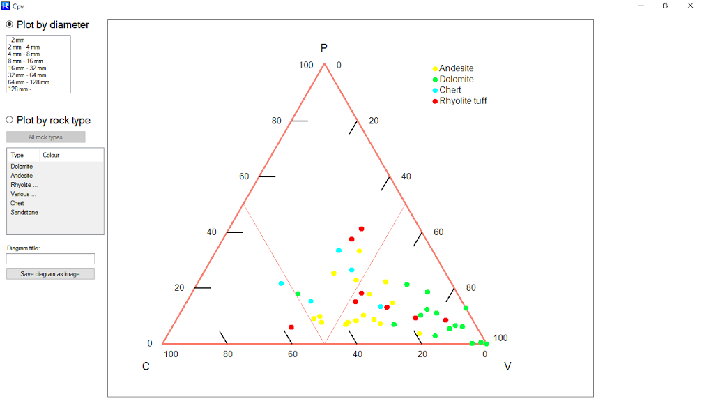
The results of CPV are presented by a graphical surface (Figure 5). Here you can see a triangle diagram. You can choose the size fraction and/or the rock types. You can name and save the diagram as image.
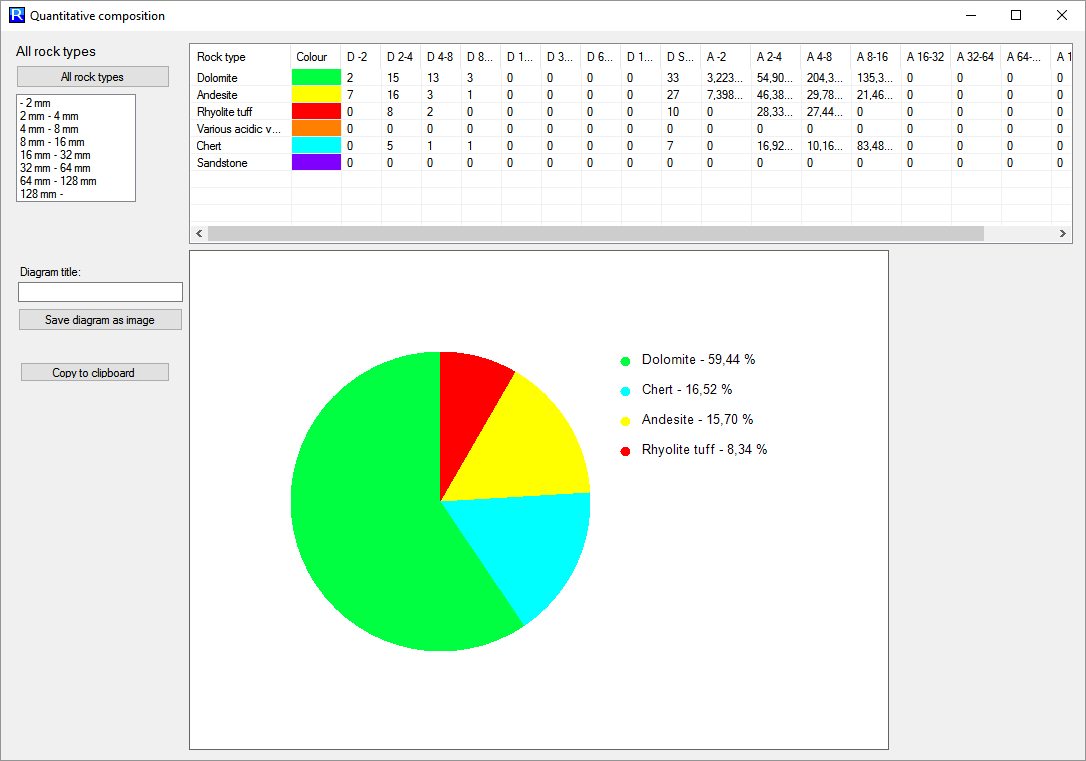
The results of the quantitative composition are presented by a graphical surface, too (Figure 6). You can see the results on a pie chart. You can choose the size fraction. You can name and save the diagram as image. You can copy the table to clipboard.
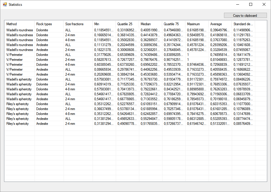
Statistics table (minimum, quartile 25, median, quartile 75, maximum, average, standard deviation) for the roundness and the sphericity (Figure 7).